How to find and select cells with conditional formatting in Google Sheets

Select 'Conditional Formatting' to locate and highlight cells with formatting rules in Google Sheets.

Why you need this tool

Managing conditional formatting rules in Google Sheets can be overwhelming, especially in large or complex spreadsheets. This tool helps you quickly find and select cells with active conditional formatting, allowing you to review or edit formatting rules with ease.

What is conditional formatting?

Conditional formatting automatically changes the appearance of cells based on predefined criteria. For example, you can highlight cells with values above a certain threshold, dates in a specific range, or text matching a particular keyword. Understanding and managing these rules is essential for maintaining clarity and accuracy in your data.

How to use the tool

First, you need to install the Select Special addon for Google Sheets. Visit the instruction page to learn how to do it step by step.

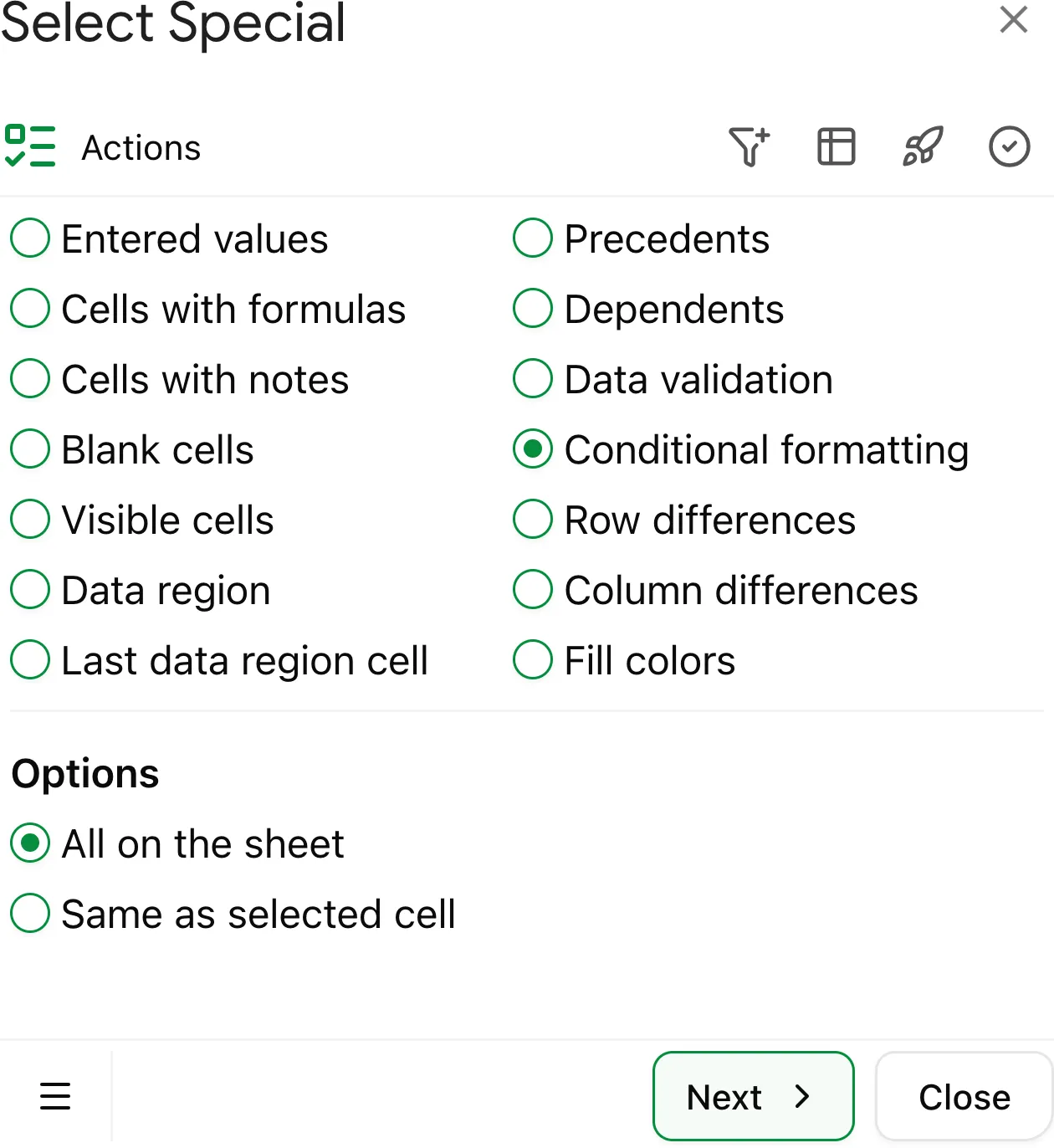
1. Select the range or scope

You can specify the scope for finding conditional formatting rules:

All on the sheet: Searches for all conditional formatting rules across the entire sheet, ensuring no rule is missed.
Same as selected cell: Searches for all conditional formatting rules identical to those applied to the currently active cell, allowing you to locate similar formatting rules quickly.

2. Execute the selection

Once the scope is defined, press the Select button in the add-on interface. The tool will select all cells with conditional formatting rules, making it simple to analyze rules as needed.